Determination of Crack Propagation Using Indirect Boundary Element Methods

Introduction

The general problem in two- or three-dimensional elastostatics is to calculate the stresses and displacements in any body under known boundary conditions. Finding analytical solutions is often quite difficult. Therefore, numerical methods have been developed. Some of these include the finite difference method, the f inite element method (FEM), and the boundary element method (BEM). The application of the boundary element method is easier for solving crack problems because calculations are performed by discretizing only the crack into linear boundary elements. Once these values are determined, the stresses and deformations in the region can be calculated.

In the boundary element method, since the solution domain of the problem is the boundaries of the region, discretization is performed on the surface of the region for three-dimensional problems and on the closed curve at the boundary of the region for two dimensional problems. Therefore, the system can be solved using fewer elements. In the Boundary Element Method, which is used for solving various engineering problems, boundary discretization is performed using two different approaches: directly or indirectly.

In the indirect boundary element method, fictitious values on the boundary are first determined. Then, these fictitious values are used to calculate the stresses and displacements in the region. In the displacement discontinuity method, displacement discontinuities are used instead of fictitious values. The displacement discontinuity method (DDM) is utilized for cracks because it allows for easier modeling in fracture mechanics problems.

In this study, crack problems were solved by combining the Fictitious Stress Method (FSM) and the Displacement Discontinuity Method (DDM). In these applications, Mode I and Mode II stress intensity factors at crack tips, as well as stresses and displacements in the cracks, were calculated, and the results were presented in tables. Crack propagation was investigated using these methods. Several numerical examples were provided, and the Stress Intensity Factor (SIF) results were compared with reference results. In this study, the entire system was solved by combining DDM and FSM solutions in the equilibrium equations. In this combined system, cracks were modeled using DDM, while other boundaries were modeled using FSM.

Obtaining Ddm And Fsm Equations

It has been observed that the use of the Displacement Discontinuity Method (DDM) has increased recently because crack problems can be more easily modeled with DDM. In deriving the displacement discontinuity equations, Papkovitch functions were used in Crouch's approach, and harmonic functions were chosen to satisfy various boundary conditions. To obtain singular solutions from dipole stresses in an isotropic medium, as done by Kimençe and Brady, derivatives of the fundamental solutions in the direction of the singular load were used.

In an infinitely elastic solid medium, at the source point P, under the influence of singular force F_i (P) , at the field point Q which is u_i (Q) , The displacement function is calculated as follows:

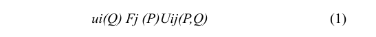
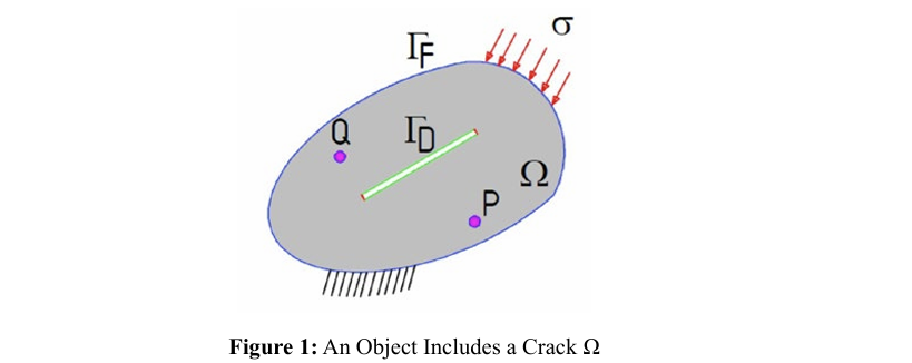
here U_ij (P,Q) this function represents the displacement in the xi direction due to the unit force applied in the xj direction. (Figure 1).

Basic solutions for DDM are given below. can be obtained as follows:

here U_ij (P,Q) this function represents the displace ment in the xi direction due to the unit force applied in the xj direction.

and stresses at any point Q due to the Fi(P) and Di(P) can be calculated as follows:

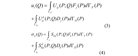
here ΓF and ΓD indicate boundaries at the surface and crack, respectively. A body and a crack in a finite plate are considered, as shown in Figure 1. Here, the boundaries are divided into constant elements of length 2a, and the stresses and displacements at the midpoint of element i are calculated due to loading on the element j. The boundary of the body and the crack is modeled using fictitious loads and displacement discontinuities. If there are a total of N elements, there are M fictitious loads along the body boundary and N-M displacement discontinuity elements along the crack. The unknown displacement discontinuities or fictitious loads are solved by summing all N elements to satisfy the boundary conditions. In the boundary element method, the boundaries are divided into N constant elements. Boundary element equations were derived by applying the boundary conditions on these elements. By solving the linear system of equations, the unknowns on the boundary were determined. Then, using these boundary unknowns, the stresses and displacements in the region were calculated. Due to the fictitious forces on element j, the i equations are as follows:

Thus, the first 2M equations in the system are obtain ed. The remaining 2(N-M) equations are derived usi ng the influence functions of the displacement disco ntinuities.

The sum of these two equations (5) and (6) can be written as follows:

here σs and σn are the tangential and normal stresses respectively. In FSM, Influence functions A_ss^ij, etc., are obtained by integrating Equation 1 over the interval (-a,a). In DDM, they are obtained by integrating Equation 6 over the interval(a,a).  Equations 5, 6, and 7 can be solved using standard numerical methods.

Determination of Stress Intensity Factors

The "stress intensity factor," K, which measures the effect of damage in a specific crack region, has been determined. Stress intensity factor values are usually normalized by the divisor K0, which corresponds to a half-length crack on an infinite surface and a crack under a normal invariant load.

In this equation, a is the half-length of the crack. Solving crack problems using both the finite element method and the boundary element method requires careful mesh design. As the number of crack tip elements increases, the rate at which the numerical solution approaches the exact solution can decrease. Various methods can be used to overcome this challenge. In this study, solutions were obtained using constant elements. Since accurate crack tip behavior can only be modeled with special elements at the crack tip, it is important to note that the length of these elements is determinative. In the boundary element method, a crack tip element with a length ranging from 0.05a to 0.2a (where a is the crack half-length) provides the best results in stress intensity factor calculations with minimal variation.

In DDM, Stress Intensity Factors (SIFs) are obtained from the displacements of the nodes around the crack tip. Through this technique, the general expressions for SIFs are given as follows:

Here, Ds and Dn are the crack opening displacements in the coordinate system associated with the examined crack tip, G is the shear modulus, ν is the Poisson's ratio, and KI and KII are the Mode I and Mode II SIFs, respectively. The coefficients k for plane stress and plane strain are given

A second-order polynomial D(ζ) has been proposed to better model the crack tip.

For the crack tip, the constants c0 and c1 on the first two (and last two) elements are obtained using displacement discontinuities, D(ξ=-a) = D1 and D(ξ=-3a)=D2 (or D(ξ=-a) = DN ve D(ξ=-3a)= DN1 Appropriate boundary influence coefficients at the midpoints of these elements can be derived in a manner similar to those for the crack tip element

In this solution approach, the SIFs were appropriately determined at ξ=-a/32.

Crack Propagation

Under LEFM conditions, crack propagation modeling requires information about two types of parameters: stress intensity factors determined analytically and the geometry as a function of load, and appropriate fracture toughness, which is an experimentally determined material property.

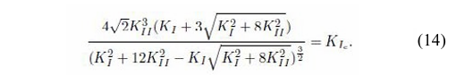
The mixed-mode stress intensity factors are calculated as Mode I and Mode II, which are the most common fracture modes in fracture mechanics. Various mixed-mode fracture criteria have been used in the literature to investigate crack initiation direction and length. Since most rocks exhibit brittle behavior under stress, the maximum tangential stress fracture criterion has been employed. Mode I fracture toughness, KIC (under plane strain conditions), is often used to predict the direction of crack propagation. This is a commonly used mixed-mode fracture mechanics criterion. According to this criterion, the crack tip will begin to propagate under the following conditions:

The following criterion is used in the maximum principal stress methods,

Crack propagation criterion

Numerical Examples

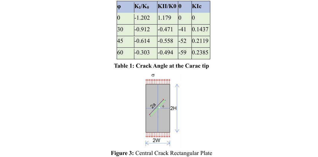
Centrally Inclined Crack Plate

A rectangular crack plate with boundary conditions shown in Figure 5 is subjected to a uniform tensile stress σ. The crack is inclined at an angle φ relative to the load direction. The ratios  are H/W=2.0 and a/W=0.5. KI and KII are calculated for various values of φ where 0<φ<π/2. The Young's modulus E is taken as 1, and the Poisson's ratio v is 0.25. In the inclined crack example, the outer boundary of the plate is divided into 48 constant FSM elements. The crack line is divided into 16 equal-length constant DDM elements. The SIFs are calculated from the crack opening displacements at a distance of approximately 0.031a from the crack tip. These SIF values are presented in a dimensionless form, SIF Kâ?? = σ√πa applied divided with the static SIF remote stress).

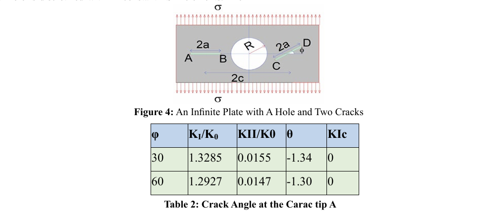
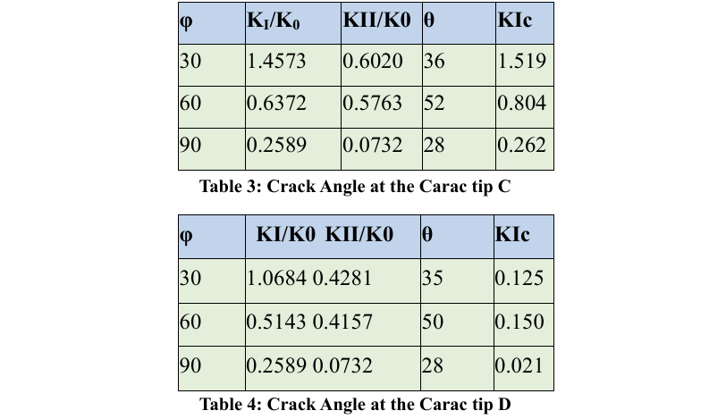
Two Crack-Circular Hole

In the second example, the geometry of the two cracks is shown in Figure 4. It is assumed that c/R=2.0, a/(c-R)=0.8 ve σ1=σ12=0, σ2=. The left crack is in a horizontal position, and the right crack is subjected to a rotation by an angle φ. The boundary of the circular hole is discretized with 24 constant FSM elements crack lines are discretized with 32 equal-length constant DDM elements. The calculated SIFs are listed in Tables 2-4. We observe that the SIFs at crack tips A and B generally change slightly when the angle φ is varied. However, the SIFs at crack tips C and D change significantly with variations in the angle φ.

Segmented Crack in a Rectangular Plate Under Tensile Stress

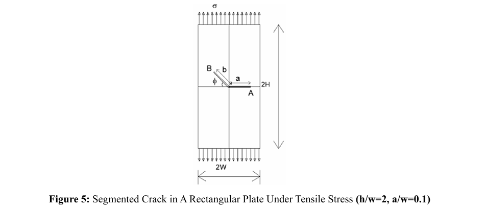
In this example, the problem of a segmented crack in a rectangular plate under tensile stress is examined, as shown in Figure 5. One segment of the crack has a horizontal length of a, while the other makes an angle of 45 degrees with the horizontal and has a length of b the horizontal representation of the entire crack 2c=a+√(2b)/2 is given. The width of the plate is shown as 2w=20 cm, and the height is 2h=40 cm.

σ=100 MPa, modulus of elasticity E=21 MPa, Poisson ratio is v=0.25. The crack is located at the center of the plate, with its height being twice its width, and the plate is subjected to a uniform tensile stress applied symmetrically at the ends. The ratios a/w=0.1 and b/a=0.2, 0.4 and 0.6 are considered, and stress intensity factors are obtained for both tips A and B. A total of 12 cases are analyzed for Modes I and II. Displacements are restrained at the ends of the rectangular plate to prevent rigid body motion.

A total of 95 boundary elements were used in the plate; the plate is discretized with 55 boundary elements along its edges. The crack is divided into 15 boundary elements at its ends—15 elements starting from crack tip B and 15 elements starting from crack tip A and 5 boundary elements in the middle—5 elements starting from crack tip B and 5 elements starting from crack tip A.

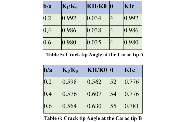
The stress intensity factors for Modes I and II at crack tips A and B were calculated using the Displacement Discontinuity Method (DDM). The computed values were compared with Murakami's results and were found to be in very good agreement.

The following tables and graphs show the comparisons of Mode I and Mode II stress intensity factors at crack tip A.

Conclusion

In this study, displacement discontinuity equations were derived using dipole solutions calculated from known singular force solutions in an isotropic medium. By combining the displacement Table 6: Crack tip Angle at the Carac tip B 6. Conclusion discontinuity method with fictitious stress methods using the solutions from these equations, various examples were solved. The formulation for obtaining displacement discontinuities in an isotropic medium using fundamental solutions has been presented. Using this formulation, various engineering problems such as tunnels and cracks have been solved.

The problem of a central inclined crack in a rectangular plate under tensile stress is solved using the combined FSM and DDM methods. The results are compared with those obtained by Wen using the equivalent stress method. It is observed that the SIFs calculated at the 0.031 point using the combined FSM-DDM formulation are in good agreement with those given by Wen.

The problem of two series cracks in an infinite region has been solved using the combined FSM and DDM methods. As shown in the tables, the stress intensity factors are compared with the values from

If the crack length is longer, modeling with only DDM is more appropriate. For longer boundary lengths, combined DDM-FSM models yield better results. While the FSM-DDM combination provides better results in the first example, modeling with DDM alone gives better results in the second example.

In conclusion, this study examined various crack problems with different geometries in finite and infinite rectangular plates under tensile stress, using the combined FSM and DDM methods in an isotropic medium. The effectiveness of the combined method was demonstrated [1-16].

References

1. Behnia, M., Goshtasbi, K., Fatehi Marji, M., & Golshani, A. (2012). On the crack propagation modeling of hydraulic fracturing by a hybridized displacement discontinuity/boundary collocation method. Journal of Mining and Environment, 2(1).

2. Schaefer, N. (2020). Predicting Fracture Extension Around a Borehole Using the Numerical Displacement Discontinuity Method. Theses and dissserations - Mining Engineering.

3. Banerjee, P. K., & Butterfield, R. (1981). Boundary element methods in engineering science.

4. Paris, F., & Canas, J. (1997). Boundary element method: fundamentals and applications.

5. Austin, M. W., Bray, J. W., & Crawford, A. M. (1982, December). A comparison of two indirect boundary element formulations incorporating planes of weakness. In International Journal of Rock Mechanics and Mining Sciences & Geomechanics Abstracts (Vol. 19, No. 6, pp. 339-344). Pergamon.

6. Crouch, S. L., & Selcuk, S. (1992, September). Two-dimensional direct boundary integral method for multilayered elastic media. In International journal of rock mechanics and mining sciences & geomechanics abstracts (Vol. 29, No. 5, pp. 491-501). Pergamon.

7. Kimençe, B., & Ergüven, M. E. (2005). Influence functions of the displacement discontinuity method for anisotropic bodies. Computational Mechanics, 36, 484-494.

8. Kimençe, B., & Ergüven, ME. (2005). Coupling of Fictitous Stress Method and Displacement Discontinuity Method for Crack Problems, 7th International Fracture Conference 19-21 October 2005, Kocaeli University, Kocaeli/ Turkey.

9. Chan, H. С. Ð?. (1993, April). Fracture mechanics analysis of the North West Fault Block of the Prudhoe Bay Field. In International journal of rock mechanics and mining sciences & geomechanics abstracts (Vol. 30, No. 2, pp. 141-149) Pergamon.

10. Civelek, M. B., & Erdogan, F. (1982). Crack problems for a rectangular plate and an infinite strip. International Journal of Fracture, 19(2), 139-159.

11. Murakami, Y. (1993). Stress Intensity Factors Handbook, Pergamon Press, Oxford.

12. Portela, A., Aliabadi, M. H., & Rooke, D. P. (1992). The dual boundary element method: effective implementation for crack problems. International journal for numerical methods in engineering, 33(6), 1269-1287.

13. Filizi, E. (2004). The Study of Cracks by The Displacement Discontinuity Method, MSc. Thesis, Department of Civil Engineering, Istanbul Technical University, Istanbul, 2004.

14. Shou, K. J., & Crouch, S. L. (1995, January). A higher order displacement discontinuity method for analysis of crack problems. In International journal of rock mechanics and mining sciences & geomechanics abstracts (Vol. 32, No. 1, pp. 49-55). Pergamon.

15. Wen, P. H. (1996). Dynamic fracture mechanics: displacement discontinuity method.

16. Chen, Y. Z., Hasabe, N., & Lee, K. Y. (2003). Multiple crack problems in elasticity.