Advancing Network Securing Strategies with Network Algorithms for Integrated Air Defense System (IADS) Missile Batteries

Keywords: Integrated Air Defense System (IADS), Network Algorithms, Network Clustering, Network Centralities, Small Worldness, Network Data Generation, Network Analysis, Big Data Computation, Regression Analysis

1. Introduction
Integrated Air Defense System (IADS) is an air defense system which is the aggregation of Service/functional component and agency Air Missile Defense (AMD) systems consist of sensors, weapons, C2, communications, intelligence systems and personnel operating in a theater or Joint Operations Area (JOA) [1]. Generally, IADS is established by Area Air Defense Commander (AADC) and, a theater AMD system in IADS typically depends on support and enabling functions from national assets and systems which are not controlled by the JFC (Joint Force Commander) [1]. As part of IADS functionality, IADS needs to provide protection of a country's assets by placing IADS missile batteries in optimal locations across the country [2]. An IADS missile battery is usually an unit of AMD which can be manually portable such as tactical air defense weapons systems or unportable such as emplaced IADS missile batteries to protect population over places which are not mobile and readily detectable based on the functionality, structure and attribute of IADS missile battery [2]. Placing an IADS missile battery over locations is a critical problem as limited IADS missile batteries are intended to protect assets over a large number of locations by considering missile ranges of IADS missile batteries for asset values over locations [2]. Locations can be represented in a network as locations are connected through real world routes or paths and on the other hand, locations can also be represented as a network where edges represent euclidean distances among locations [2]. But in case of missile range, euclidean distances among locations need to be considered as edges for representing a location network. In case of placing IADS missile batteries in a network, optimal location nodes need to be found, for that, aa huge number of network algorithms existed in literature such as network algorithms based on the sum of the fraction of all-pairs shortest paths, the reciprocal of the average shortest path distance, the structure of incoming links, the centrality of neighbors, the sum of the fraction of all-pairs shortest paths, etc [3-9].

In this research, a model for sequential development of seven strategies with the use of six network algorithms has been introduced.These weighted edge location networks with generated assigned values are basically generated by using Watts Strogatz graph algorithm, which is based on small worldness, computed with network clustering coefficient algorithm [10-13]. The results that came from after applying seven strategies to generated location networks have been analyzed with ordinary least square linear regression analysis at the end.

2. Methodology and Computational Experiment
For developing sequential model of seven network securing strategies, six network algorithms have been selected to measure each node of the location networks, where network_algorithm_1 is based on the sum of the fraction of all-pairs shortest paths , network_algorithm_2 is based on the reciprocal of the average shortest path distance, network_algorithm_3 is a ranking of nodes in graph based on the structure of incoming links, network_algorithm_4 is based on the centrality of neighbors, network_algorithm_5 is based on the sum of the fraction of all-pairs shortest paths similar to network_algorithm_1, and network_algorithm_6 is measuring a node as the fraction of nodes that it is connected to [3-9]. These network algorithms have been used to develop a sequential developing model of seven network securing strategies in section 4 named as “Strategies”.

To generate weighted edge location networks with assigned asset values, Watts Strogatz small world network generation algorithm has been selected where assigned asset values (see Figure 4) are following power law distribution [10-11][2]. Besides considering Euclidean distances, it is assumed that to hit each location’s attacker missile, the interceptor missiles have different flying altitudes and different trajectory paths which doesn’t depend on Euclidean distance because of geographical attributes such as hills, mountains, etc. For that reason, the trajectory path distance of an interceptor missile has been considered as range for that interceptor missile.Because of considering different flying altitudes' trajectory paths as distances among nodes, generated location networks don't follow Pythagorean theorem or Euclidean theorem [27-28].

As a scale of small worldness, five types of small worldness have been selected for generating 20 networks of 50 location nodes with different diameters where small worldness is close to zero means more to small world characteristics [11].

By applying seven strategies upon previously generated 20 location networks with 50 nodes, total unprotected asset value percentages (Worst Case Scenarios) have been computed for each strategy with 98% of IADS missile battey’s interceptor missile’s interceptor probability [15]. To analyze the result that came from applying seven strategies upon generated location networks, ordinary least square linear regression analysis has been used for analyzing relations among sum of all IADS missile ranges, network diameters of generated location networks and unprotected asset value percentages for optimal strategy of each generated network [14]. Besides that, ordinary least square linear regression analysis has also been used for analyzing relations among sum of all IADS missile ranges, network diameters of generated location networks and small worldness for optimal strategy of each generated network [14].

3. Computational Instruments
Python 3 Google Compute Engine has been used where System RAM is 12.7 GB and Disk is 107.7 GB [16]. Code has been written in Python language and Packages are: Google.colab: 0.0.1a2, Networkx: 3.0, Pandas: 1.3.5, Numpy: 1.21.6, Matplotlib: 3.5.3, Scipy: 1.10.0, Array, Statsmodels.api: 0.13.5, Sklearn: 1.2.1 [17-24]. Documentation done in Google Docs [29].

4. Strategies
In this section, seven network securing strategies have been developed with six network algorithms which have been introduced in the Methodology section.

Strategy_1:
Step 1. Considering weighted edge network with asset values for placing IADS's batteries
Step 2. Computing network_algorithm_1
Step 3. Putting IADS missile battery with maximum interceptor missile range on the place of first maximum network_algorithm_1 measure and if second IADS missile battery exists with with maximum interceptor missile range or less than interceptor missile range then, putting the second IADS missile battery on the place of the next maximum network_algorithm_1 measure where distance from the node of first maximum network_algorithm_1 measure is more than maximum IADS missile battery interceptor missile range.
Step 4. And doing the same for placing rest of IADS batteries on next maximum network_algorithm_1 measure where node distance from first placed IADS missile battery is more than first IADS battery’s interceptor missile range For example, one generated weighted edge location network has been introduced below. One, two and three IADS missile batteries have been applied sequentially on that generated weighted edge location network where interceptor missile ranges are sequentially 80 km, 70 km and 20 km.

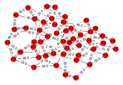
Figure 1: Weighted edge network with asset values. Each asset value is scored as a fraction number (between 0.0 and 1.0) out of 1. All nodes are unprotected (colored as red) as no IADS missile battery has been placed. Here, The diameter of network is 180 km

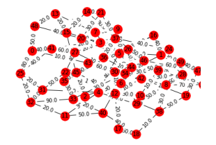
Figure 2: Weighted edge network with location node numbers. All nodes are unprotected (colored as red) as no IADS missile battery has been placed. Here, The diameter of network is 180 km

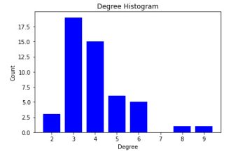
Figure 3: Degree distribution histogram of weighted edge network

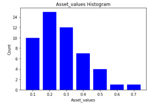
Figure 4: Asset value distribution histogram of weighted edge network

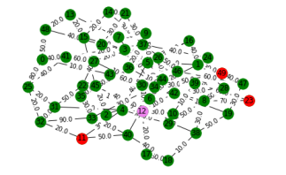
Figure 5: Violet nodes are where IADS missile batteries have been placed and red nodes are unprotected location node numbers where IADS missile battery’s interceptor missiles can't reach. One IADS missile battery is placed at location node number 12. Placed IADS missile battery’s interceptor missile range is 80 km Here, total unprotected asset value is 0.5

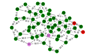
Figure 6: Violet nodes are where IADS missile batteries have been placed and red nodes are unprotected location node numbers where IADS missile battery’s interceptor missiles can't reach. First IADS missile battery is placed at location node number 12 and Second IADS missile battery is placed at location node number 11. First placed IADS missile battery’s interceptor missile range is 80 km and second placed IADS missile battery’s interceptor missile range is 70 km. Here, total unprotected asset value is 0.4

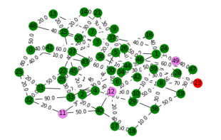
Figure 7: Violet nodes are where IADS missile batteries have been placed and red nodes are unprotected location node numbers where IADS missile battery’s interceptor missiles can't reach. First IADS missile battery is placed at location node 12, Second IADS missile battery is placed at location node 11 and Third IADS missile battery is placed at location node 49. First placed IADS missile battery’s interceptor missile range is 80 km, second placed IADS missile battery’s interceptor missile range is 70 km and third placed IADS missile battery’s interceptor missile range is 20 km. Here, total unprotected asset value is 0.2

Strategy_2:
(Same as Strategy_1 except using network_algorithm_2 instead of network_algorithm_1)
Step 1. Considering weighted edge network with asset values for placing IADS's batteries
Step 2. Computing network_algorithm_2
Step 3. Putting IADS missile battery with maximum interceptor missile range on the place of first maximum network_algorithm_2 measure and if second IADS missile battery exists with with maximum interceptor missile range or less than interceptor missile range then, putting the second IADS missile battery on the place of the next maximum network_algorithm_2 measure where distance from the node of first maximum network_algorithm_2 measure is more than maximum IADS missile battery interceptor missile range.
Step 4. And doing the same for placing rest of IADS batteries on next maximum network_algorithm_2 measure where node distance from first placed IADS missile battery is more than first IADS battery’s interceptor missile range [26-29].

For example, One, two and three IADS missile batteries have been applied sequentially on that previously generated weighted edge location network where interceptor missile ranges are sequentially 80 km, 70 km and 20 km.

Figure 8: Violet nodes are where IADS missile batteries have been placed and red nodes are unprotected location node numbers where IADS missile battery’s interceptor missiles can't reach. One IADS missile battery is placed at location node number 5. Placed IADS missile battery’s interceptor missile range is 80 km Here, total unprotected asset value is 2.3000000000000003

Figure 9: Violet nodes are where IADS missile batteries have been placed and red nodes are unprotected location node numbers where IADS missile battery’s interceptor missiles can't reach. First IADS missile battery is placed at location node 5 and Second IADS missile battery is placed at location node 34. First placed IADS missile battery’s interceptor missile range is 80 km and second placed IADS missile battery’s interceptor missile range is 70 km. Here, total unprotected asset value is 0.5

Figure 10: Violet nodes are where IADS missile batteries have been placed and red nodes are unprotected location node numbers where IADS missile battery’s interceptor missiles can't reach. First IADS missile battery is placed at location node 5, Second IADS missile battery is placed at location node 34 and Third IADS missile battery is placed at location node 39. First placed IADS missile battery’s interceptor missile range is 80 km, second placed IADS missile battery’s interceptor missile range is 70 km and third placed IADS missile battery’s interceptor missile range is 20 km. Here, total unprotected asset value is 0.5

Strategy_3:
Step 1. Considering weighted edge network with asset values for placing IADS's batteries.
Step 2. Computing network_algorithm_1, network_algorithm_2, network_algorithm_3, network_algorithm_4, network_
algorithm_5 and network_algorithm_6.
Step 3. Creating six sequences by ordering location node numbers as descending orders of the results of six network algorithms sequentially such as sequence_number_1 is the sequence of node numbers ordered as descending order of network_algorithm_1’s measuring values on nodes.
Step 4. Estimating total unprotected asset values for placing IADS missile battery with maximum missile range on the place of first location node number from each sequence and choosing the lowest unprotected asset value corresponded node among six unprotected asset value corresponded nodes for placing first IADS with maximum missile range.

Step 5. Estimating total unprotected asset values for placing second IADS missile battery (if any) with maximum missile range or with second maximum missile range on the place of second location node number from each sequence and choosing the lowest unprotected asset value corresponded location node among six unprotected asset value corresponded location nodes for placing second IADS with maximum missile range or with second maximum missile range. If the lowest unprotected asset value corresponded location node resulted from considering second node position of each sequence is same as the lowest unprotected asset value corresponded node resulted from considering first node position of each sequence, then repeat step 4 for the place of third location node number in sequences for placing second IADS missile battery with maximum missile range or with second maximum missile range.

Step 6. Repeating Step_4 and Step_5 for placing the next IADS missile battery with previous missile ranges or with the next longer missile range (which is less than previous missile range).
Lowest unprotected asset;value corresponded location node
Step 7. If there are number of nodes where the resulted from considering any node position of each sequence is same as the lowest unprotected asset value corresponded node resulted from considering previous node number of IADS batteries with previous missile ranges; or position of each sequence, then,for placing the last with the the most minimum missile ranges, detect all unprotected location nodes where previously placed IADS batteries interceptor missiles can't reach.
Step 8. Estimating total unprotected asset values for unprotected location▭node and choosing the lowest total placing the last number of IADS batteries on each unprotected location nodes for placing the▭last ▭number of unprotected asset value corresponding to number of IADS batteries with previous missile ranges or with the most minimum missile ranges.

For example, One, two and three IADS missile batteries have been applied sequentially on that previously generated weighted edge location network where interceptor missile ranges are sequentially 80 km, 70 km and 20 km.

Figure 11: Violet nodes are where IADS missile batteries have been placed and red nodes are unprotected location node numbers where IADS missile battery’s interceptor missiles can't reach. One IADS missile battery is placed at location node number 12. Placed IADS missile battery’s interceptor missile range is 80 km Here, total unprotected asset value is 0.

Figure 12: Violet nodes are where IADS missile batteries have been placed and red nodes are unprotected location node numbers where IADS missile battery’s interceptor missiles can't reach. First IADS missile battery is placed at location node number 12 and Second IADS missile battery is placed at location node number 11. First placed IADS missile battery’s interceptor missile range is 80 km and second placed IADS missile battery’s interceptor missile range is 70 km. Here, total unprotected asset value is 0.4

Figure 13: Violet nodes are where IADS missile batteries have been placed and red nodes are unprotected location node numbers where IADS missile battery’s interceptor missiles can't reach. First IADS missile battery is placed at location node 12, Second IADS missile battery is placed at location node 22 and Third IADS missile battery is placed at location node 11. First placed IADS missile battery’s interceptor missile range is 80 km, second placed IADS missile battery’s interceptor missile range is 70 km and third placed IADS missile battery’s interceptor missile range is 20 km. Here, total unprotected asset value is 0.4

Strategy 4:
(Same as Strategy_3 for first four steps)
Step 1. Considering weighted edge network with asset values for placing IADS's batteries
Step 2. Computing network_algorithm_1, network_algorithm_2, network_algorithm_3, network_algorithm_4, network_algorithm_5 and network_algorithm_6
Step 3. Creating six sequences by ordering location node numbers as descending orders of the results of six network algorithms sequentially such as sequence_number_1 is the sequence of node numbers ordered as descending order of network_algorithm_1’s measuring values on nodes.
Step 4. Estimating total unprotected asset values for placing IADS missile battery with maximum missile range on the place of first location node number from each sequence and choosing the lowest unprotected asset value corresponded node among six unprotected asset value corresponded nodes for placing first IADS with maximum missile range.
Step 5. After placing the first IADS missile battery with maximum missile range, for placing the next IADS missile batteries, we shall consider those location nodes in six sequences where the distances from the first placed IADS missile battery are more than the first placed IADS missile battery’s missile range.
Step 6. Repeating Step_4 for placing the next IADS missile battery with previous missile ranges or with the next longer missile range (which is less than previous missile range) until all IADS missile batteries are placed. If the lowest unprotected asset value corresponded location node resulted from considering any node position of each sequence is same as the lowest unprotected asset value corresponded node resulted from considering previous node position of each sequence, then, we shall consider the second lowest unprotected asset value corresponded location node resulted from considering that node position of each sequence for placing IADS missile battery.

For example, One, two and three IADS missile batteries have been applied sequentially on that previously generated weighted edge location network where interceptor missile ranges are sequentially 80 km, 70 km and 20 km.

Figure 14: Violet nodes are where IADS missile batteries have been placed and red nodes are unprotected location node numbers where IADS missile battery’s interceptor missiles can't reach. One IADS missile battery is placed at location node number 12. Placed IADS missile battery’s interceptor missile range is 80 km Here, total unprotected asset value is 0.5

Figure 15: Violet nodes are where IADS missile batteries have been placed and red nodes are unprotected location node numbers where IADS missile battery’s interceptor missiles can't reach. First IADS missile battery is placed at location node number 12 and Second IADS missile battery is placed at location node number 34. First placed IADS missile battery’s interceptor missile range is 80 km and second placed IADS missile battery’s interceptor missile range is 70 km. Here, total unprotected asset value is 0.30000000000000004

Figure 16: Violet nodes are where IADS missile batteries have been placed and red nodes are unprotected location node numbers where IADS missile battery’s interceptor missiles can't reach. First IADS missile battery is placed at location node 12, Second IADS missile battery is placed at location node 34 and Third IADS missile battery is placed at location node 39. First placed IADS missile battery’s interceptor missile range is 80 km, second placed IADS missile battery’s interceptor missile range is 70 km and third placed IADS missile battery’s interceptor missile range is 20 km. Here, total unprotected asset value is 0.30000000000000004

Strategy_5:
(Same as Strategy_3 and Strategy_4 for first four steps)
Step 1. Considering weighted edge network with asset values for placing IADS's batteries
Step 2. Computing network_algorithm_1, network_algorithm_2, network_algorithm_3, network_algorithm_4, network_algorithm_5 and network_algorithm_6
Step 3. Creating six sequences by ordering location node numbers as descending orders of the results of six network algorithms sequentially such as sequence_number_1 is the sequence of node numbers ordered as descending order of network_algorithm_1’s measuring values on nodes.
Step 4. Estimating total unprotected asset values for placing IADS missile battery with maximum missile range on the place of first location node number from each sequence and choosing the lowest unprotected asset value corresponded node among six unprotected asset value corresponded nodes for placing first IADS with maximum missile range.
Step 5. After placing the first IADS missile battery with maximum missile range, we shall estimate total unprotected asset values (but for this strategy, unlike Strategy_3, we shall consider only those unprotected asset values which are not protected by previously placed IADS missile batteries) for placing next IADS missile battery with maximum missile range or with the rest of minimum missile ranges on the place of the next location node number where the distances from the first placed IADS missile battery is more than the first placed IADS missile battery’s missile range in each sequence and choosing the lowest unprotected asset value corresponded location node among six unprotected asset value corresponded location nodes for placing the next IADS with maximum missile range or with the rest of minimum missile ranges.
Step 6. Repeating Step 5 for placing the next IADS missile battery with previous missile ranges or with the next longer missile range (which is less than previous missile range) until all IADS missile batteries are placed.

For example, One, two and three IADS missile batteries have been applied sequentially on that previously generated weighted edge location network where interceptor missile ranges are sequentially 80 km, 70 km and 20 km.

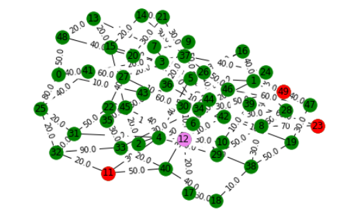
Figure 17: Violet nodes are where IADS missile batteries have been placed and red nodes are unprotected location node numbers where IADS missile battery’s interceptor missiles can't reach. One IADS missile battery is placed at location node number 12. Placed IADS missile battery’s interceptor missile range is 80 km Here, total unprotected asset value is 0.5

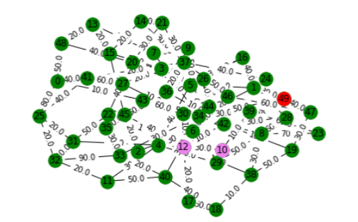
Figure 18: Violet nodes are where IADS missile batteries have been placed and red nodes are unprotected location node numbers where IADS missile battery’s interceptor missiles can't reach. First IADS missile battery is placed at location node number 12 and Second IADS missile battery is placed at location node number 10. First placed IADS missile battery’s interceptor missile range is 80 km and second placed IADS missile battery’s interceptor missile range is 70 km. Here, total unprotected asset value is 0.2

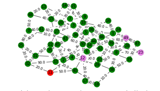
Figure 19: Violet nodes are where IADS missile batteries have been placed and red nodes are unprotected location node numbers where IADS missile battery’s interceptor missiles can't reach. First IADS missile battery is placed at location node 12, Second IADS missile battery is placed at location node 23 and third IADS missile battery is placed at location node 49.

First placed IADS missile battery’s interceptor missile range is 80 km, second placed IADS missile battery’s interceptor missile range is 70 km and third placed IADS missile battery’s interceptor missile range is 20 km. Here, total unprotected asset value is 0.1

Strategy 6:
(Same as Strategy_3 and Strategy_4 for first four steps)
Step 1. Considering weighted edge network with asset values for placing IADS's batteries
Step 2. Computing network_algorithm_1, network_algorithm_2, network_algorithm_3, network_algorithm_4, network_algorithm_5 and network_algorithm_6
Step 3. Creating six sequences by ordering location node numbers as descending orders of the results of six network algorithms sequentially such as sequence_number_1 is the sequence of node numbers ordered as descending order of network_algorithm_1’s measuring values on nodes.
Step 4. Estimating total unprotected asset values for placing IADS missile battery with maximum missile range on the place of first location node number from each sequence and choosing the lowest unprotected asset value corresponded node among six unprotected asset value corresponded nodes for placing first IADS with maximum missile range.
Step 5. After placing first IADS missile battery, we shall choose nodes from longest shortest distance path from first placed IADS missile battery and shortest path between previous shortest distance end node (end node of shortest distance path from first placed IADS missile battery) and first placed IADS missile battery location node.
Step 6. Including that, we shall choose nodes from shortest distance path between network diameter source node and first placed IADS_mssle_battery's location node and we shall also choose nodes from shortest distance path between network diameter target node and first placed IADS missile battery’s location node.
Step 7. Creating sequence of chosen nodes without any order of ascending or descending and, from that sequence, we shall select optimal location nodes for placing the rest of IADS missile batteries based on less unprotected asset value cost as per rest of IADS missile batteries ranges.

For example, One, two and three IADS missile batteries have been applied sequentially on that previously generated weighted edge location network where interceptor missile ranges are sequentially 80 km, 70 km and 20 km.

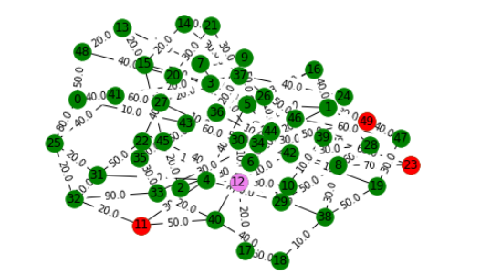
Figure 20: Violet nodes are where IADS missile batteries have been placed and red nodes are unprotected location node numbers where IADS missile battery’s interceptor missiles can't reach. One IADS missile battery is placed at location node number 12. Placed IADS missile battery’s interceptor missile range is 80 km Here, total unprotected asset value is 0.5

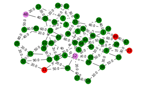
Figure 21: Violet nodes are where IADS missile batteries have been placed and red nodes are unprotected location node numbers where IADS missile battery’s interceptor missiles can't reach. First IADS missile battery is placed at location node number 12 and Second IADS missile battery is placed at location node number 48. First placed IADS missile battery’s interceptor missile range is 80 km and second placed IADS missile battery’s interceptor missile range is 70 km. Here, total unprotected asset value is 0.5

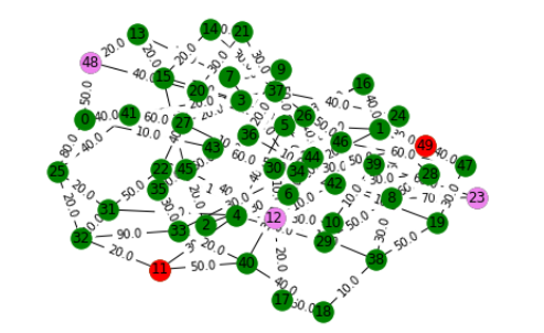
Figure 22: Violet nodes are where IADS missile batteries have been placed and red nodes are unprotected location node numbers where IADS missile battery’s interceptor missiles can't reach. First IADS missile battery is placed at location node 12, Second IADS missile battery is placed at location node 48 and third IADS missile battery is placed at location node 23.

First placed IADS missile battery’s interceptor missile range is 80 km, second placed IADS missile battery’s interceptor missile range is 70 km and third placed IADS missile battery’s interceptor missile range is 20 km. Here, total unprotected asset value is 0.30000000000000004

Strategy_7:
(same as Strategy_3 and Strategy_4 for first four steps)
Step_1. Considering weighted edge network with asset values for placing IADS's batteries
Step_2. Computing network_algorithm_1, network_algorithm_2, network_algorithm_3, network_algorithm_4, network_algorithm_5 and network_algorithm_6
Step_3. Creating six sequences by ordering location node numbers as descending orders of the results of six network algorithms sequentially such as sequence_number_1 is the sequence of node numbers ordered d scending order of network_algorithm_1’s measuring values on odes.
Step_4. Estimating total unprotected asset values for placing IADS missile battery with maximum missile range on the place of first location node number from each sequence and choosing the lowest unprotected asset value corresponded node among six unprotected asset value corresponded nodes for placing first IADS with maximum missile range.
Step_5. After placing first IADS missile battery, we shall choose nodes from longest shortest distance path from first placed IADS missile battery and shortest path between previous shortest distance end node (end node of shortest distance path from first placed IADS missile battery) and first placed IADS missile battery location node.
Step_6. Including that, we shall choose nodes from shortest distance path between network diameter source node and first placed IADS_mssle_battery's location node and we shall also choose nodes from shortest distance path between network diameter target node and first placed IADS missile battery’s location node.
Step_7. Creating sequence of chosen nodes without any order of ascending or descending and from that sequence, creating another sequence from betweenness centrality subset of previously created subset.
Step_8. From the last created sequence, we shall select optimal location nodes for placing the rest of IADS missile batteries based on less unprotected asset value cost as per rest of IADS missile batteries ranges.

For example, One, two and three IADS missile batteries have been applied sequentially on that previously generated weighted edge location network where interceptor missile ranges are sequentially 80 km, 70 km and 20 km.

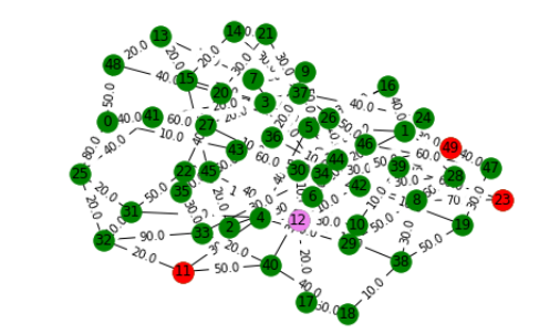
Figure 23: Violet nodes are where IADS missile batteries have been placed and red nodes are unprotected location node numbers where IADS missile battery’s interceptor missiles can't reach. One IADS missile battery is placed at location node number 12. Placed IADS missile battery’s interceptor missile range is 80 km Here, total unprotected asset value is 0.5

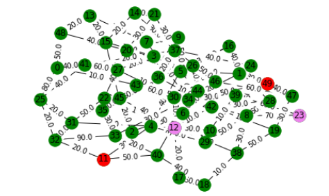
Figure 24: Violet nodes are where IADS missile batteries have been placed and red nodes are unprotected location node numbers where IADS missile battery’s interceptor missiles can't reach. First IADS missile battery is placed at location node number 12 and Second IADS missile battery is placed atlocation node number 23. First placed IADS missile battery’s interceptor missile range is 80 km and second placed IADS missile battery’s interceptor missile range is 70 km. Here, total unprotected asset value is 0.30000000000000004

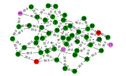
Figure 25: Viol nodes are where IADS missile batteries have been placed and red nodes are unprotected location node numbers where IADS missile battery’s interceptor missiles can't reach. First IADS missile battery is placed at location node 12, Second IADS missile battery is placed at location node 23 and third IADS missile battery is placed at location node 48. First placed IADS missile battery’s interceptor missile range is 80 km, second placed IADS missile battery’s interceptor missile range is 70 km and third placed IADS missile batt ry’s interceptor missile range is 20 km. Here, total unprotected asset value is 0.30000000000000004

First placed IADS missile battery’s interceptor missile range is 80 km, second placed IADS missile battery’s interceptor missile range is 70 km and third placed IADS missile battery’s interceptor missile range is 20 km. Here, total unprotected asset value is 0.30000000000000004

5. COMPUTATIONAL RESULTS
Table 1 has been created for results of two IADS missile batteries where interceptor missile battery ranges

Strategy number	Generated weighted edge location network’s small worldness	Generated weighted edge location network’s node number	Generated weighted edge location network’s Diameter	Generated weighted edge location network’s Minimum edge length and Maximum edge length (Minimum, Maximum)	Generated weighted edge location network total asset value	IADS missile batteries Interceptor missile ranges in kilometer	IADS missile batteries interceptor missile’s interceptor probability	After placing IADS missile batteries, total Unprotected asset value	After placing IADS missile batteries, total Unprotected asset value Percentage (Worst Case Scenario )
Strategy_1	≈0.39692	50	123.0 km	(20.5 km, 184.5 km)	≈14.9	80 km, 70 km	98%	1.6	≈12.52349%
Strategy_2	≈0.39692	50	123.0 km	(20.5 km, 184.5 km)	≈14.9	80 km, 70 km	98%	1.6	≈12.52349%
Strategy_3	≈0.39692	50	123.0 km	(20.5 km, 184.5 km)	≈14.9	80 km, 70 km	98%	0.6	≈5.94631%
Strategy_4	≈0.39692	50	123.0 km	(20.5 km, 184.5 km)	≈14.9	80 km, 70 km	98%	1.8	≈13.83893%
Strategy_5	≈0.39692	50	123.0 km	(20.5 km, 184.5 km)	≈14.9	80 km, 70 km	98%	0.2	≈3.315436%
Strategy_6	≈0.39692	50	123.0 km	(20.5 km, 184.5 km)	≈14.9	80 km, 70 km	98%	1.0	≈8.577181%
Strategy_7	≈0.39692	50	123.0 km	(20.5 km, 184.5 km)	≈14.9	80 km, 70 km	98%	1.0	≈8.577181%
Strategy_1	≈0.582777	50	133.0 km	(19 km, 171.0 km)	≈14.4	80 km, 70 km	98%	0.3	≈4.0416667%
Strategy_2	≈0.582777	50	133.0 km	(19 km, 171.0 km)	≈14.4	80 km, 70 km	98%	0.3	≈4.0416667%
Strategy_3	≈0.582777	50	133.0 km	(19 km, 171.0 km)	≈14.4	80 km, 70 km	98%	0.9	≈8.1250000%
Strategy_4	≈0.582777	50	133.0 km	(19 km, 171.0 km)	≈14.4	80 km, 70 km	98%	0.4	≈4.7222222%
Strategy_5	≈0.582777	50	133.0 km	(19 km, 171.0 km)	≈14.4	80 km, 70 km	98%	0.2	≈3.3611111%
Strategy_6	≈0.582777	50	133.0 km	(19 km, 171.0 km)	≈14.4	80 km, 70 km	98%	0.3	≈4.0416667%
Strategy_7	≈0.582777	50	133.0 km	(19 km, 171.0 km)	≈14.4	80 km, 70 km	98%	0.3	≈4.0416667%
Strategy_1	≈0.640091	50	200.0 km	(20.0 km, 160.0 km)	≈14.3	80 km, 70 km	98%	4.1	≈30.097902%
Strategy_2	≈0.640091	50	200.0 km	(20.0 km, 160.0 km)	≈14.3	80 km, 70 km	98%	4.5	≈32.839161%
Strategy_3	≈0.640091	50	200.0 km	(20.0 km, 160.0 km)	≈14.3	80 km, 70 km	98%	3.3	≈24.615385%
Strategy_4	≈0.640091	50	200.0 km	(20.0 km, 160.0 km)	≈14.3	80 km, 70 km	98%	1.3	≈10.90909%
Strategy_5	≈0.640091	50	200.0 km	(20.0 km, 160.0 km)	≈14.3	80 km, 70 km	98%	1.3	≈10.90909%
Strategy_6	≈0.640091	50	200.0 km	(20.0 km, 160.0 km)	≈14.3	80 km, 70 km	98%	2.7	≈20.503497%
Strategy_7	≈0.640091	50	200.0 km	(20.0 km, 160.0 km)	≈14.3	80 km, 70 km	98%	2.4	≈18.447552%
Strategy_1	≈0.807039	50	710.0 km	(10 km, 70 km)	≈15.4	80 km, 70 km	98%	10.5	≈68.181818%
Strategy_2	≈0.807039	50	710.0 km	(10 km, 70 km)	≈15.4	80 km, 70 km	98%	12.5	≈81.545455%
Strategy_3	≈0.807039	50	710.0 km	(10 km, 70 km)	≈15.4	80 km, 70 km	98%	7.2	≈47.818182%
Strategy_4	≈0.807039	50	710.0 km	(10 km, 70 km)	≈15.4	80 km, 70 km	98%	10.6	≈69.454545%
Strategy_5	≈0.807039	50	710.0 km	(10 km, 70 km)	≈15.4	80 km, 70 km	98%	6.6	≈44.00%
Strategy_6	≈0.807039	50	710.0 km	(10 km, 70 km)	≈15.4	80 km, 70 km	98%	6.6	≈44.00%
Strategy_7	≈0.807039	50	710.0 km	(10 km, 70 km)	≈15.4	80 km, 70 km	98%	6.6	≈44.00%
Strategy_1	≈1.145887	50	560.0 km	(10 km, 80 km)	≈14.1	80 km, 70 km	98%	9.2	≈65.943262%
Strategy_2	≈1.145887	50	560.0 km	(10 km, 80 km)	≈14.1	80 km, 70 km	98%	9.2	≈65.943262%
Strategy_3	≈1.145887	50	560.0 km	(10 km, 80 km)	≈14.1	80 km, 70 km	98%	8.4	≈60.382979%
Strategy_4	≈1.145887	50	560.0 km	(10 km, 80 km)	≈14.1	80 km, 70 km	98%	8.4	≈60.382979%
Strategy_5	≈1.145887	50	560.0 km	(10 km, 80 km)	≈14.1	80 km, 70 km	98%	7.9	≈56.907801%
Strategy_6	≈1.145887	50	560.0 km	(10 km, 80 km)	≈14.1	80 km, 70 km	98%	8.4	≈60.382979%
Strategy_7	≈1.145887	50	560.0 km	(10 km, 80 km)	≈14.1	80 km, 70 km	98%	7.9	≈56.907801%

Table 1: Results for two IADS missile batteries where interceptor missile battery ranges are sequentially 80 km and 70 km where worst case scenario’s unprotected asset value percentages (including calculating interceptor missile’s interceptor probabilities by considering only one IADS missile battery’s one interceptor missile for one attacker missile) have been listed for each of few generated weighted edge networks and for each strategy.

Table 2 has been created for results for three IADS missile batteries where interceptor missile battery ranges are sequentially 110 km, 90 km and 80 km where worst case scenario’s unprotected asset value percentages (Including calculating interceptor missile’s interceptor probabilities by considering only one IADS missile battery’s one interceptor missile for one attacker missile) have been listed for few generated weighted edge networks and for each strategy.

Strategy number	Generated weighted edge location network’s small worldness	Generated weighted edge location network’s node number	Generated weighted edge location network’s Diameter	Generated weighted edge location network’s Minimum edge length and Maximum edge length (Minimum, Maximum)	Generated weighted edge location network total asset value	IADS missile batteries Interceptor missile ranges in kilometer	IADS missile batteries interceptor missile’s interceptor probability	After placing IADS missile batteries, total Unprotected asset value	After placing IADS missile batteries, total Unprotected asset value Percentage (Worst Case Scenario )
Strategy_1	≈0.423134	50	210.0 km	(35 km, 315 km)	13.8	110 km, 90 km, 80 km	98%	0.9	≈8.39130%
Strategy_2	≈0.423134	50	210.0 km	(35 km, 315 km)	13.8	110 km, 90 km, 80 km	98%	1.0	≈9.101449%
Strategy_3	≈0.423134	50	210.0 km	(35 km, 315 km)	13.8	110 km, 90 km, 80 km	98%	0.6	≈6.26087%
Strategy_4	≈0.423134	50	210.0 km	(35 km, 315 km)	13.8	110 km, 90 km, 80 km	98%	0.1	≈2.71014%
Strategy_5	≈0.423134	50	210.0 km	(35 km, 315 km)	13.8	110 km, 90 km, 80 km	98%	0.0	2.0%
Strategy_6	≈0.423134	50	210.0 km	(35 km, 315 km)	13.8	110 km, 90 km, 80 km	98%	0.4	≈4.84058%
Strategy_7	≈0.423134	50	210.0 km	(35 km, 315 km)	13.8	110 km, 90 km, 80 km	98%	0.4	≈4.84058%
Strategy_1	≈0.564176	50	270.0 km	(18 km, 144 km)	15.0	110 km, 90 km, 80 km	98%	4.7	≈32.706667%
Strategy_2	≈0.564176	50	270.0 km	(18 km, 144 km)	15.0	110 km, 90 km, 80 km	98%	5.5	≈37.933333%
Strategy_3	≈0.564176	50	270.0 km	(18 km, 144 km)	15.0	110 km, 90 km, 80 km	98%	4.7	≈32.706667%
Strategy_4	≈0.564176	50	270.0 km	(18 km, 144 km)	15.0	110 km, 90 km, 80 km	98%	2.1	≈15.72%
Strategy_5	≈0.564176	50	270.0 km	(18 km, 144 km)	15.0	110 km, 90 km, 80 km	98%	2.1	≈15.72%
Strategy_6	≈0.564176	50	270.0 km	(18 km, 144 km)	15.0	110 km, 90 km, 80 km	98%	4.5	≈31.4%
Strategy_7	≈0.564176	50	270.0 km	(18 km, 144 km)	15.0	110 km, 90 km, 80 km	98%	4.5	≈31.4%
Strategy_1	≈0.640606	50	200.0 km	(25 km, 225 km)	15.7	110 km, 90 km, 80 km	98%	0.3	≈3.872611%
Strategy_2	≈0.640606	50	200.0 km	(25 km, 225 km)	15.7	110 km, 90 km, 80 km	98%	1.1	≈8.866242%
Strategy_3	≈0.640606	50	200.0 km	(25 km, 225 km)	15.7	110 km, 90 km, 80 km	98%	2.4	≈16.980891%
Strategy_4	≈0.640606	50	200.0 km	(25 km, 225 km)	15.7	110 km, 90 km, 80 km	98%	1.1	≈8.866242%
Strategy_5	≈0.640606	50	200.0 km	(25 km, 225 km)	15.7	110 km, 90 km, 80 km	98%	0.1	≈2.6242038%
Strategy_6	≈0.640606	50	200.0 km	(25 km, 225 km)	15.7	110 km, 90 km, 80 km	98%	1.0	≈8.2420382%
Strategy_7	≈0.640606	50	200.0 km	(25 km, 225 km)	15.7	110 km, 90 km, 80 km	98%	1.0	≈8.2420382%
Strategy_1	≈0.829442	50	345.0 km	(23 km, 184 km)	15.4	110 km, 90 km, 80 km	98%	5.1	≈34.454545%
Strategy_2	≈0.829442	50	345.0 km	(23 km, 184 km)	15.4	110 km, 90 km, 80 km	98%	8.9	≈58.636363%
Strategy_3	≈0.829442	50	345.0 km	(23 km, 184 km)	15.4	110 km, 90 km, 80 km	98%	8.0	≈52.909090%
Strategy_4	≈0.829442	50	345.0 km	(23 km, 184 km)	15.4	110 km, 90 km, 80 km	98%	4.1	≈28.090909%
Strategy_5	≈0.829442	50	345.0 km	(23 km, 184 km)	15.4	110 km, 90 km, 80 km	98%	3.5	≈24.272727%
Strategy_6	≈0.829442	50	345.0 km	(23 km, 184 km)	15.4	110 km, 90 km, 80 km	98%	5.8	≈38.90909%
Strategy_7	≈0.829442	50	345.0 km	(23 km, 184 km)	15.4	110 km, 90 km, 80 km	98%	6.2	≈41.454545%
Strategy_1	≈1.16390	50	960.0 km	(20 km, 160 km)	14.2	110 km, 90 km, 80 km	98%	10.5	≈74.464789%
Strategy_2	≈1.16390	50	960.0 km	(20 km, 160 km)	14.2	110 km, 90 km, 80 km	98%	10.8	≈76.535211%
Strategy_3	≈1.16390	50	960.0 km	(20 km, 160 km)	14.2	110 km, 90 km, 80 km	98%	10.8	≈76.535211%
Strategy_4	≈1.16390	50	960.0 km	(20 km, 160 km)	14.2	110 km, 90 km, 80 km	98%	10.3	≈73.084507%
Strategy_5	≈1.16390	50	960.0 km	(20 km, 160 km)	14.2	110 km, 90 km, 80 km	98%	9.4	≈66.873239%
Strategy_6	≈1.16390	50	960.0 km	(20 km, 160 km)	14.2	110 km, 90 km, 80 km	98%	10.2	≈72.394366%
Strategy_7	≈1.16390	50	960.0 km	(20 km, 160 km)	14.2	110 km, 90 km, 80 km	98%	11.2	≈79.295775%

Table 2: Results for three IADS missile batteries where interceptor missile battery ranges are sequentially 110 km, 90 km and 80 km where worst case scenario’s unprotected asset value percentages (including calculating interceptor missile’s interceptor probabilities by considering only one IADS missile battery’s one interceptor missile for one attacker missile) have been listed for each of few generated weighted edge networks and for each strategy. Table 3 has been created for results for four IADS missile batteries where interceptor missile battery ranges are sequentially 120 km, 110 km, 90 km and 80 km where worst case scenario’s unprotected asset value percentages

Table 3 has been created for results for four IADS missile batteries where interceptor missile battery ranges are sequentially 120 km, 110 km, 90 km and 80 km where worst case scenario’s unprotected asset value percentages

Strategy number	Generated weighted edge location network’s small worldness	Generated weighted edge location network’s node number	Generated weighted edge location network’s Diameter	Generated weighted edge location network’s Minimum edge length and Maximum edge length (Minimum, Maximum)	Generated weighted edge location network total asset value	IADS missile batteries Interceptor missile ranges in kilometer	IADS missile batteries interceptor missile’s interceptor probability	After placing IADS missile batteries, total Unprotected asset value	After placing IADS missile batteries, total Unprotected asset value Percentage (Worst Case Scenario )
Strategy_1	≈0.25351	50	270.0 km	(45 km, 405 km)	14.1	120 km, 110 km 90 km, 80 km	98%	2.4	≈18.68085%
Strategy_2	≈0.25351	50	270.0 km	(45 km, 405 km)	14.1	120 km, 110 km 90 km, 80 km	98%	3.8	≈28.4113%
Strategy_3	≈0.25351	50	270.0 km	(45 km, 405 km)	14.1	120 km, 110 km 90 km, 80 km	98%	1.7	≈13.8156%
Strategy_4	≈0.25351	50	270.0 km	(45 km, 405 km)	14.1	120 km, 110 km 90 km, 80 km	98%	1.4	≈11.730%
Strategy_5	≈0.25351	50	270.0 km	(45 km, 405 km)	14.1	120 km, 110 km 90 km, 80 km	98%	0.3	≈4.0851%
Strategy_6	≈0.25351	50	270.0 km	(45 km, 405 km)	14.1	120 km, 110 km 90 km, 80 km	98%	1.9	≈15.20567%
Strategy_7	≈0.25351	50	270.0 km	(45 km, 405 km)	14.1	120 km, 110 km 90 km, 80 km	98%	1.6	≈13.120567%
Strategy_1	≈0.405311	50	360.0 km	(60 km, 540 km)	13.2	120 km, 110 km 90 km, 80 km	98%	4.9	≈38.378788%
Strategy_2	≈0.405311	50	360.0 km	(60 km, 540 km)	13.2	120 km, 110 km 90 km, 80 km	98%	6.9	≈53.227272%
Strategy_3	≈0.405311	50	360.0 km	(60 km, 540 km)	13.2	120 km, 110 km 90 km, 80 km	98%	6.2	≈48.030303%
Strategy_4	≈0.405311	50	360.0 km	(60 km, 540 km)	13.2	120 km, 110 km 90 km, 80 km	98%	5.7	≈44.318181%
Strategy_5	≈0.405311	50	360.0 km	(60 km, 540 km)	13.2	120 km, 110 km 90 km, 80 km	98%	5.3	≈41.34848%
Strategy_6	≈0.405311	50	360.0 km	(60 km, 540 km)	13.2	120 km, 110 km 90 km, 80 km	98%	7.7	≈59.2%
Strategy_7	≈0.405311	50	360.0 km	(60 km, 540 km)	13.2	120 km, 110 km 90 km, 80 km	98%	5.6	≈43.575757%
Strategy_1	≈0.652449	50	375.0 km	(25 km, 200 km)	16.2	120 km, 110 km 90 km, 80 km	98%	5.2	≈33.45679%
Strategy_2	≈0.652449	50	375.0 km	(25 km, 200 km)	16.2	120 km, 110 km 90 km, 80 km	98%	4.6	≈29.82716%
Strategy_3	≈0.652449	50	375.0 km	(25 km, 200 km)	16.2	120 km, 110 km 90 km, 80 km	98%	3.0	≈20.14815%
Strategy_4	≈0.652449	50	375.0 km	(25 km, 200 km)	16.2	120 km, 110 km 90 km, 80 km	98%	3.6	≈23.7778%
Strategy_5	≈0.652449	50	375.0 km	(25 km, 200 km)	16.2	120 km, 110 km 90 km, 80 km	98%	1.5	≈11.074074%
Strategy_6	≈0.652449	50	375.0 km	(25 km, 200 km)	16.2	120 km, 110 km 90 km, 80 km	98%	5.1	≈32.85185%
Strategy_7	≈0.652449	50	375.0 km	(25 km, 200 km)	16.2	120 km, 110 km 90 km, 80 km	98%	4.7	≈30.4321%
Strategy_1	≈0.934170	50	697.0 km	(17 km, 119 km)	14.6	120 km, 110 km 90 km, 80 km	98%	6.7	≈46.9726%
Strategy_2	≈0.934170	50	697.0 km	(17 km, 119 km)	14.6	120 km, 110 km 90 km, 80 km	98%	8.6	≈59.7260%
Strategy_3	≈0.934170	50	697.0 km	(17 km, 119 km)	14.6	120 km, 110 km 90 km, 80 km	98%	6.8	≈47.64383%
Strategy_4	≈0.934170	50	697.0 km	(17 km, 119 km)	14.6	120 km, 110 km 90 km, 80 km	98%	5.7	≈40.26027%
Strategy_5	≈0.934170	50	697.0 km	(17 km, 119 km)	14.6	120 km, 110 km 90 km, 80 km	98%	3.0	≈22.136986%
Strategy_6	≈0.934170	50	697.0 km	(17 km, 119 km)	14.6	120 km, 110 km 90 km, 80 km	98%	3.1	≈22.8082%
Strategy_7	≈0.934170	50	697.0 km	(17 km, 119 km)	14.6	120 km, 110 km 90 km, 80 km	98%	4.0	≈28.849315%
Strategy_1	≈1.11291	50	960.0 km	(15 km, 135 km)	16.1	120 km, 110 km 90 km, 80 km	98%	9.7	≈61.043478%
Strategy_2	≈1.11291	50	960.0 km	(15 km, 135 km)	16.1	120 km, 110 km 90 km, 80 km	98%	10.3	≈64.695652%
Strategy_3	≈1.11291	50	960.0 km	(15 km, 135 km)	16.1	120 km, 110 km 90 km, 80 km	98%	11.4	≈71.39130%
Strategy_4	≈1.11291	50	960.0 km	(15 km, 135 km)	16.1	120 km, 110 km 90 km, 80 km	98%	11.8	≈73.826089%
Strategy_5	≈1.11291	50	960.0 km	(15 km, 135 km)	16.1	120 km, 110 km 90 km, 80 km	98%	7.0	≈44.608696%
Strategy_6	≈1.11291	50	960.0 km	(15 km, 135 km)	16.1	120 km, 110 km 90 km, 80 km	98%	9.7	≈61.043478%
Strategy_7	≈1.11291	50	960.0 km	(15 km, 135 km)	16.1	120 km, 110 km 90 km, 80 km	98%	10.0	≈62.869565%

Table 3: Results for four IADS missile batteries where interceptor missile battery ranges are sequentially 120 km, 110 km, 90 km and 80 km where worst case scenario’s unprotected asset value percentages (including calculating interceptor missile’s interceptor probabilities by considering only one IADS missile battery’s one interceptor missile for one attacker missile) have been listed for each of few generated weighted edge networks and for each strategy.

Table 4 has been created for results for five IADS missile batteries where interceptor missile battery ranges are sequentially 200 km, 120 km, 110 km, 90 km and 80 km where worst case scenario’s unprotected asset value percentages (including calculating interceptor missile’s interceptor probabilities by considering only one IADS missile battery’s one interceptor missile for one attacker missile) have been listed for few generated weighted edge networks and for each strategy.

Strategy number	Generated weighted edge location network’s small worldness	Generated weighted edge location network’s node number	Generated weighted edge location network’s Diameter	Generated weighted edge location network’s Minimum edge length and Maximum edge length (Minimum, Maximum)	Generated weighted edge location network total asset value	IADS missile batteries Interceptor missile ranges in kilometer	IADS missile batteries interceptor missile’s interceptor probability	After placing IADS missile batteries, total Unprotected asset value	After placing IADS missile batteries, total Unprotected asset value Percentage (Worst Case Scenario )
Strategy_1	≈0.344096	50	480.0 km	(80.0 km, 640.0 km)	16.2	200 km, 120 km 110 km 90 km, 80 km	98%	3.3	≈21.96296%
Strategy_2	≈0.344096	50	480.0 km	(80.0 km, 640.0 km)	16.2	200 km, 120 km 110 km 90 km, 80 km	98%	3.8	≈24.987654%
Strategy_3	≈0.344096	50	480.0 km	(80.0 km, 640.0 km)	16.2	200 km, 120 km 110 km 90 km, 80 km	98%	4.5	≈29.2222%
Strategy_3	≈0.344096	50	480.0 km	(80.0 km, 640.0 km)	16.2	200 km, 120 km 110 km 90 km, 80 km	98%	4.5	≈29.2222%
Strategy_4	≈0.344096	50	480.0 km	(80.0 km, 640.0 km)	16.2	200 km, 120 km 110 km 90 km, 80 km	98%	3.8	≈24.98765%
Strategy_5	≈0.344096	50	480.0 km	(80.0 km, 640.0 km)	16.2	200 km, 120 km 110 km 90 km, 80 km	98%	2.3	≈15.91358%
Strategy_6	≈0.344096	50	480.0 km	(80.0 km, 640.0 km)	16.2	200 km, 120 km 110 km 90 km, 80 km	98%	4.0	≈26.19753%
Strategy_7	≈0.344096	50	480.0 km	(80.0 km, 640.0 km)	16.2	200 km, 120 km 110 km 90 km, 80 km	98%	3.7	≈24.382716%
Strategy_1	≈0.431319	50	375.0 km	(75.0 km, 675.0 km)	14.7	200 km, 120 km 110 km 90 km, 80 km	98%	8.6	≈59.333%
Strategy_2	≈0.431319	50	375.0 km	(75.0 km, 675.0 km)	14.7	200 km, 120 km 110 km 90 km, 80 km	98%	10.5	72.0%
Strategy_3	≈0.431319	50	375.0 km	(75.0 km, 675.0 km)	14.7	200 km, 120 km 110 km 90 km, 80 km	98%	5.3	≈37.3333%
Strategy_4	≈0.431319	50	375.0 km	(75.0 km, 675.0 km)	14.7	200 km, 120 km 110 km 90 km, 80 km	98%	4.4	≈31.333%
Strategy_5	≈0.431319	50	375.0 km	(75.0 km, 675.0 km)	14.7	200 km, 120 km 110 km 90 km, 80 km	98%	2.6	≈19.33333%
Strategy_6	≈0.431319	50	375.0 km	(75.0 km, 675.0 km)	14.7	200 km, 120 km 110 km 90 km, 80 km	98%	7.3	≈50.66667%
Strategy_7	≈0.431319	50	375.0 km	(75.0 km, 675.0 km)	14.7	200 km, 120 km 110 km 90 km, 80 km	98%	4.6	≈32.6666%
Strategy_1	≈0.652398	50	550.0 km	(50.0 km, 400.0 km)	15.3	200 km, 120 km 110 km 90 km, 80 km	98%	5.5	≈37.228758%
Strategy_2	≈0.652398	50	550.0 km	(50.0 km, 400.0 km)	15.3	200 km, 120 km 110 km 90 km, 80 km	98%	6.9	≈46.196078%
Strategy_3	≈0.652398	50	550.0 km	(50.0 km, 400.0 km)	15.3	200 km, 120 km 110 km 90 km, 80 km	98%	6.4	≈42.993464%
Strategy_4	≈0.652398	50	550.0 km	(50.0 km, 400.0 km)	15.3	200 km, 120 km 110 km 90 km, 80 km	98%	4.7	≈32.104575%
Strategy_5	≈0.652398	50	550.0 km	(50.0 km, 400.0 km)	15.3	200 km, 120 km 110 km 90 km, 80 km	98%	2.6	≈18.65359%
Strategy_6	≈0.652398	50	550.0 km	(50.0 km, 400.0 km)	15.3	200 km, 120 km 110 km 90 km, 80 km	98%	6.8	≈45.555556%
Strategy_7	≈0.652398	50	550.0 km	(50.0 km, 400.0 km)	15.3	200 km, 120 km 110 km 90 km, 80 km	98%	5.1	≈34.666667%
Strategy_1	≈0.880917	50	600.0 km	(40.0 km, 360.0 km)	14.7	200 km, 120 km 110 km 90 km, 80 km	98%	4.9	≈34.666667%
Strategy_2	≈0.880917	50	600.0 km	(40.0 km, 360.0 km)	14.7	200 km, 120 km 110 km 90 km, 80 km	98%	6.7	≈46.666667%
Strategy_3	≈0.880917	50	600.0 km	(40.0 km, 360.0 km)	14.7	200 km, 120 km 110 km 90 km, 80 km	98%	5.5	≈38.666667%
Strategy_4	≈0.880917	50	600.0 km	(40.0 km, 360.0 km)	14.7	200 km, 120 km 110 km 90 km, 80 km	98%	4.4	≈31.33333%
Strategy_5	≈0.880917	50	600.0 km	(40.0 km, 360.0 km)	14.7	200 km, 120 km 110 km 90 km, 80 km	98%	1.8	14.0%
Strategy_6	≈0.880917	50	600.0 km	(40.0 km, 360.0 km)	14.7	200 km, 120 km 110 km 90 km, 80 km	98%	6.5	≈45.333333%
Strategy_7	≈0.880917	50	600.0 km	(40.0 km, 360.0 km)	14.7	200 km, 120 km 110 km 90 km, 80 km	98%	5.7	≈40.00%
Strategy_1	≈1.12557	50	1425.0 km	(25.0 km, 250.0 km)	14.0	200 km, 120 km 110 km 90 km, 80 km	98%	6.5	≈47.5%
Strategy_2	≈1.12557	50	1425.0 km	(25.0 km, 250.0 km)	14.0	200 km, 120 km 110 km 90 km, 80 km	98%	7.9	≈57.3%
Strategy_3	≈1.12557	50	1425.0 km	(25.0 km, 250.0 km)	14.0	200 km, 120 km 110 km 90 km, 80 km	98%	7.5	≈54.5%
Strategy_4	≈1.12557	50	1425.0 km	(25.0 km, 250.0 km)	14.0	200 km, 120 km 110 km 90 km, 80 km	98%	7.1	≈51.7%
Strategy_5	≈1.12557	50	1425.0 km	(25.0 km, 250.0 km)	14.0	200 km, 120 km 110 km 90 km, 80 km	98%	4.1	≈30.7%
Strategy_6	≈1.12557	50	1425.0 km	(25.0 km, 250.0 km)	14.0	200 km, 120 km 110 km 90 km, 80 km	98%	6.6	≈48.2%
Strategy_7	≈1.12557	50	1425.0 km	(25.0 km, 250.0 km)	14.0	200 km, 120 km 110 km 90 km, 80 km	98%	6.9	≈50.3%

Table 4 Results for five IADS missile batteries where interceptor missile battery ranges are sequentially 200km, 120 km, 110 km, 90 km and 80 km where worst case scenario’s unprotected asset value percentages (including calculating interceptor missile’s interceptor probabilities by considering only one IADS missile battery’s one interceptor missile for one attacker missile) have been listed for each of few generated weighted edge networks and for each strategy.

By aggregating each optimal solution for each generated network, we found Table 5.

 

Strategy number	Generated weighted edge location network’s small worldness	Generated weighted edge location network’s node number	Generated weighted edge location network’s Diameter	Generated weighted edge location network’s Minimum edge length and Maximum edge length (Minimum, Maximum)	Generated weighted edge location network total asset value	IADS missile batteries Interceptor missile ranges in kilometer	IADS missile batteries interceptor missile’s interceptor probability	After placing IADS missile batteries, total Unprotected asset value	After placing IADS missile batteries, total Unprotected asset value Percentage (Worst Case Scenario )
Strategy_5	≈0.39692	50	123.0 km	(20.5 km, 184.5 km)	≈14.9	80 km, 70 km	98%	0.2	≈3.315436%
Strategy_5	≈0.582777	50	133.0 km	(19 km, 171.0 km)	≈14.4	80 km, 70 km	98%	0.2	≈3.3611111%
Strategy_5	≈0.640091	50	200.0 km	(20.0 km, 160.0 km)	≈14.3	80 km, 70 km	98%	1.3	≈10.90909%
Strategy_5 or, Strategy_6 or, Strategy_7	≈0.807039	50	710.0 km	(10 km, 70 km)	≈15.4	80 km, 70 km	98%	6.6	≈44.00%
Strategy_5	≈1.145887	50	560.0 km	(10 km, 80 km)	≈14.1	80 km, 70 km	98%	7.9	≈56.907801%
Strategy_5	≈0.423134	50	210.0 km	(35 km, 315 km)	≈13.8	110 km 90 km, 80 km	98%	0.0	2.0%
Strategy_4 or Strategy_5	≈0.564176	50	270.0 km	(18 km, 144 km)	≈15.0	110 km 90 km, 80 km	98%	2.1	≈15.72%
Strategy_5	≈0.640606	50	200.0 km	(25 km, 225 km)	≈15.7	110 km 90 km, 80 km	98%	0.1	≈2.6242038%
Strategy_5	≈0.829442	50	345.0 km	(23 km, 184 km)	≈15.4	110 km 90 km, 80 km	98%	3.5	≈24.272727%
Strategy_5	≈1.1639	50	960.0 km	(20 km, 160 km)	14.2	110 km 90 km, 80 km	98%	9.4	≈66.873239%
Strategy_5	≈0.25351	50	270.0 km	(45 km, 405 km)	14.1	120 km 110 km, 90 km 80 km	98%	0.3	≈4.0851%
Strategy_5	≈0.405311	50	360.0 km	(60 km, 540 km)	13.2	120 km, 110 km, 90 km, 80 km	98%	5.3	≈41.34848%
Strategy_5	≈0.652449	50	375.0 km	(25 km, 200 km)	16.2	120 km 110 km, 90 km 80 km	98%	1.5	≈11.074074%
Strategy_5	≈0.934170	50	697.0 km	(17 km, 119 km)	14.6	120 km 110 km, 90 km 80 km	98%	3.0	≈22.136986%
Strategy_5	≈1.11291	50	960.0 km	(15 km, 135 km)	16.1	120 km 110 km, 90 km 80 km	98%	7.0	≈44.608696%
Strategy_5	≈0.344096	50	480.0 km	(80.0 km, 640.0 km)	16.2	200 km 120 km 110 km, 90 km 80 km	98%	2.3	≈15.91358%
Strategy_5	≈0.431319	50	375.0 km	(75.0 km, 675.0 km)	14.7	200 km 120 km 110 km, 90 km 80 km	98%	2.6	≈19.33333%
Strategy_5	≈0.652398	50	550.0 km	(50.0 km, 400.0 km)	15.3	200 km 120 km 110 km, 90 km 80 km	98%	2.6	≈18.65359%
Strategy_5	≈0.880917	50	600.0 km	(40.0 km, 360.0 km)	14.7	200 km 120 km 110 km, 90 km 80 km	98%	1.8	14.0%
Strategy_5	≈1.12557	50	1425.0 km	(25.0 km, 25.0 km)	14.0	200 km 120 km 110 km, 90 km 80 km	98%	4.1	≈30.7%

 

Table 5: Aggregation of optimal solution for each generated network

Ordinary Least Square Linear Regression analysis (Figure 26) of Table 5 where dependent variable is generated weighted edge location network’s small worldness and independent variables are generated weighted edge location network diameter and sum of IADS missile batteries interceptor missile ranges. Here, R-squared is ≈0.7, coefficient of generated weighted edge location network diameter is 0.0008, coefficient of sum of IADS missile batteries interceptor missile ranges is -0.0007 and constant is 0.5615

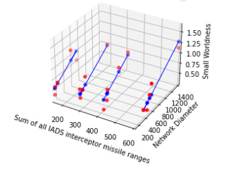
Figure 26: 3D Depiction of Table 5’s linear regression analysis for each sum of IADS missile batteries interceptor missile ranges where sum of IADS missile batteries interceptor missile ranges are sequentially 150 km, 280 km, 400 km and 600 km. Red dots are training data, blue dots are predicted data and blue lines are linear regression lines for each sum of IADS missile batteries interceptor missile ranges.

Ordinary Least Square Linear Regression analysis (Figure 27) of Table 5 where dependent variable is total unprotected asset value percentage and independent variables are generated weighted edge location network diameter and sum of IADS missile batteries interceptor missile ranges. Here, R-squared is ≈0.6, coefficient of generated weighted edge location network diameter is 0.0463, coefficient of sum of IADS missile batteries interceptor missile ranges is -0.0440 and constant is 15.6197

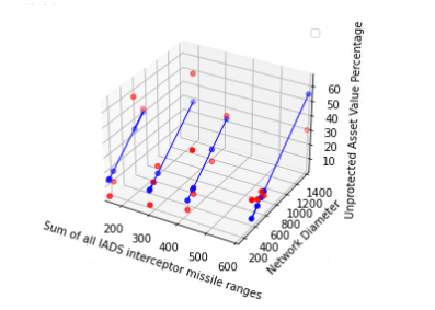
Figure 27: 3D Depiction of Table 5’s linear regression analysis for each sum of IADS missile batteries interceptor missile ranges where sum of IADS missile batteries interceptor missile ranges are sequentially 150 km, 280 km, 400 km and 600 km. Red dots are training data, blue dots are predicted data and blue lines are linear regression lines for each sum of IADS missile batteries interceptor missile ranges.

6. CONCLUSION
As it is found from computational results that Strategy_5 is the most optimal strategy for small world networks and networks which are not small world networks. In some cases, Strategy_4, Strategy_6 and Strategy_7 are also optimal strategies along with Strategy_5. Eventually, by analyzing computational results, it can be stated that Strategy_6 and Strategy_7 tend to be optimal when the location network has less small world characteristics and the diameter is far longer than the sum of all IADS missile batteries interceptor missile ranges. On the other hand, Strategy_4 tends to be optimal when the location network has more small world characteristics and the diameter is equal or less than the sum of all IADS missile batteries interceptor missile ranges. From regression analysis, it can be stated that, with increasing the location network diameter and the sum of all IADS missile batteries interceptor missile ranges, small worldness value of the location network for optimal strategy also increases (more small world value means less small world characteristics) and, with increasing the location network diameter and the sum of all IADS missile batteries interceptor missile ranges, total unprotected asset value percentages (worst case scenario) of the location network for optimal strategy also increases.

For future research, we may consider scale-free networks as location networks and in place of regression analysis we may use other supervised learning methods such as artificial neural networks to understand relationship patterns among location networks properties and IADS missile battery’s interceptor missile’s properties [25-26].

References

1. Air Countering and Missile Threats (2017). "Joint Publication 3-01." United States Joint Chief of Staff: Washington, DC, USA.

2. Han, C. Y., Lunday, B. J., & Robbins, M. J. (2016). A game theoretic model for the optimal location of integrated air
defense system missile batteries. INFORMS Journal on Computing, 28(3), 405-416.

3. Brandes, U. (2001). A faster algorithm for betweenness centrality. Journal of mathematical sociology, 25(2), 163-177.

4. Brandes, U. (2008). On variants of shortest-path betweenness centrality and their generic computation. Social networks, 30(2), 136-145.

5. Freeman, L. C. (1979). Centrality in social networks: Conceptual clarification. Social network: critical concepts in sociology. Londres: Routledge, 1, 238-263.

6. Stanley, W., & Katherine, F. (1994). Social network analysis: Methods and applications. Cambridge: Cambridge University.

7. Langville, A. N., & Meyer, C. D. (2005). A survey of eigenvector methods for web information retrieval. SIAM review, 47(1), 135-161.

8. Bonacich, P. (1986). Power and centrality: A family of measures. American journal of sociology, 92(5), 1170-1182.

9. Newman, M. E. (2001). Scientific collaboration networks. II. Shortest paths, weighted networks, and centrality. Physical review E, 64(1), 016132.

10. Duncan, J. Watts, and Steven, H. (1998). Strogatz, Collective dynamics of small-world networks, Nature, 393, pp. 440–442.

11. Telesford, Q. K., Joyce, K. E., Hayasaka, S., Burdette, J. H., & Laurienti, P. J. (2011). The ubiquity of small-world networks.

12. Saramäki, J., Kivelä, M., Onnela, J. P., Kaski, K., & Kertesz, J. (2007). Generalizations of the clustering coefficient to weighted complex networks. Physical Review E, 75(2), 027105.

13. Kaiser, M. (2008). Mean clustering coefficients: the role of isolated nodes and leafs on clustering measures for small-world networks. New Journal of Physics, 10(8), 083042.

14. Hutcheson, G. D., & Moutinho, L. A. M. (2011). The SAGE dictionary of quantitative management research. The SAGE Dictionary of Quantitative Management Research, 1-344.

15. Wilkening, D. A. (2000). A simple model for calculating ballistic missile defense effectiveness. Science & Global Security, 8(2), 183-215.

16. Sanderson, D. (2015). Programming Google App Engine with Python: Build and Run Scalable Python Apps on Google's Infrastructure. " O'Reilly Media, Inc”.

17. Summerfield, M. (2010). Programming in Python 3: a omplete introduction to the Python language. Addison-Wesley Professional.

18. Hagberg, A., Swart, P., & S Chult, D. (2008). Exploring network structure, dynamics, and function using NetworkX (No. LA-UR-08-05495; LA-UR-08-5495). Los Alamos National Lab.(LANL), Los Alamos, NM (United States).

19. McKinney, W. (2011). pandas: a foundational Python library for data analysis and statistics. Python for high performance and scientific computing, 14(9), 1-9.

20. McKinney, W. (2012). Python for data analysis: Data wrangling with Pandas, NumPy, and IPython. " O'Reilly Media, Inc."

21. Ari, Niyazi., and Makhamadsulton, Ustazhanov. (2014). "Matplotlib in python." 2014 11th International Conference on Electronics, Computer and Computation (ICECCO). IEEE.

22. Virtanen, P., Gommers, R., Oliphant, T. E., Haberland, M., Reddy, T., Cournapeau, D., & Van Mulbregt, P. (2020). SciPy 1.0: fundamental algorithms for scientific computing in Python. Nature methods, 17(3), 261-272.

23. McKinney, W., Perktold, J., & Seabold, S. (2011). Time series analysis in python with statsmodels. Jarrodmillman Com, 96-102.

24. Pedregosa, Fabian. (2011). et al. "Scikit-learn: Machine learning in Python." the Journal of machine Learning research 12 (2011): 2825-2830.

25. Barabási, A. L. (2009). Scale-free networks: a decade and beyond. science, 325(5939), 412-413.

26. Pran, R. H., & Todorovski, L. (2021). Predicting Hidden Links and Missing Nodes in Scale-Free Networks with Artificial Neural Networks. arXiv preprint arXiv:2109.12331.

27. Kadison, R. V. (2002). The Pythagorean Theorem: I. The finite case. Proceedings of the National Academy of Sciences, 99(7), 4178-4184.

28. Finney, R. L. (1970). Dynamic proofs of Euclidean theorems. Mathematics Magazine, 43(4), 177-185.

29. Attebury, R., George, J., Judd, C., & Marcum, B. (2008). Google docs: a review. Against the Grain, 20(2), 9.
 

Copyright: ©2023 Rakib Hassan Pran. This is an open-access article distributed under the terms of the Creative Commons Attribution License, which permits unrestricted use, distribution, and reproduction in any medium, provided the original author and source are credited.